Data analysis

In the current version of PHYLOViZ, you can analyze your data using the several algorithms described below. Press the Right Mouse Button on the Typing Data (now named with the method) and choose compute to access the available analysis algorithms.

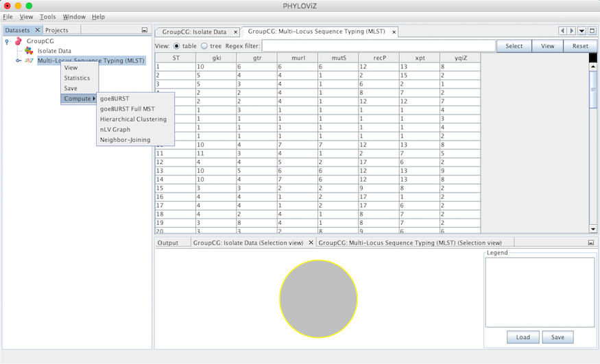
goeBURST algorithm

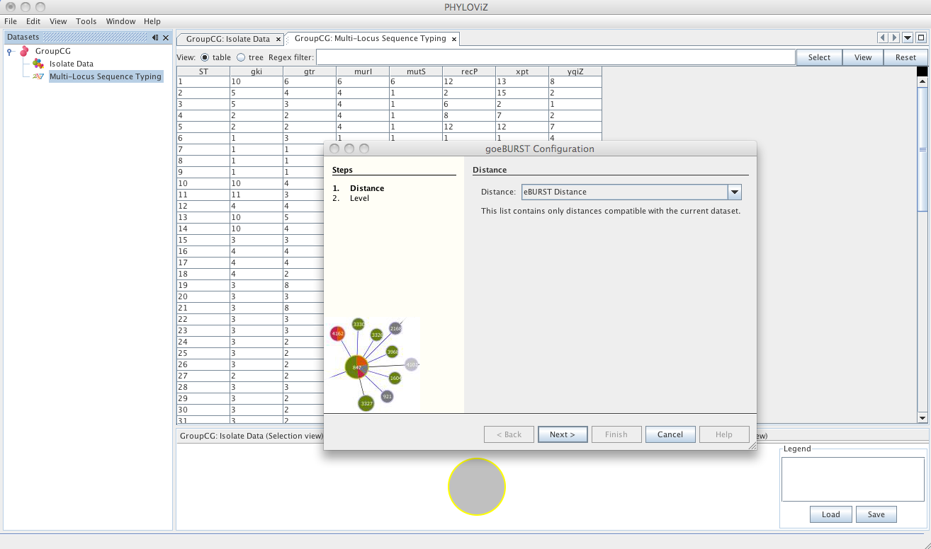
Selecting the goeBURST algorithms opens the dialog for the goeBURST algorithm. This algorithm was typically used for MLST data analysis and was originally described in the article Global optimal eBURST analysis of multilocus typing data using a graphic matroid approach. The first step is choosing the Distance to be used. Currently eBURST Distance is the only one available, but others could be implemented. The eBURST distances follows the tiebreak rules discussed in the article.

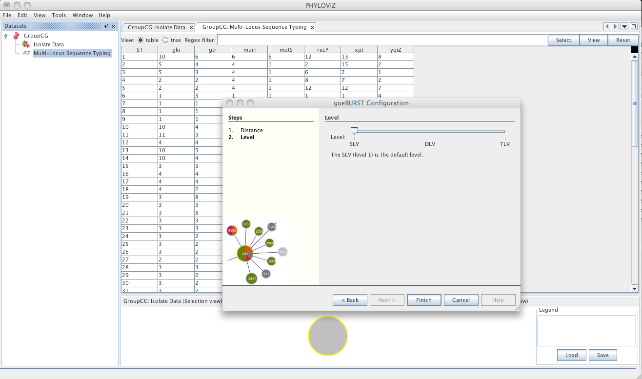
The second step is the choice of the level to which clonal complexes will be formed. The usual default for MLST analysis is SLV Level. Choosing DLV or TLV level will take longer calculation times, but could provide some insight to the relationships between clonal complexes formed at SLV and DLV level respectively.

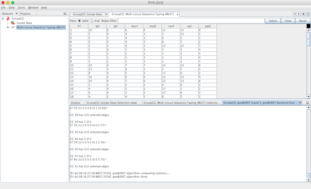
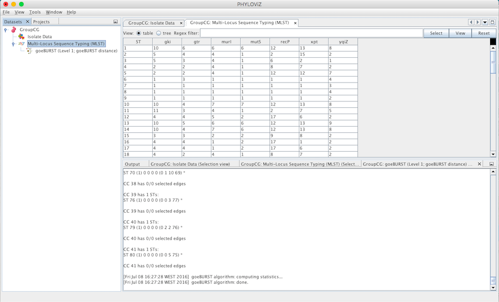
A goeBURST Output tab will appear and display the goeBURST algorithm results. It will contain information about the Clonal Complexes (CCs), namely the Sequence Types that compose them and what edges (the links between STs) were drawn in each CC.

In order to display the goEburst tree view, it is necessary to expand the typing data on the DataSets’ tab, if it is not already expanded.

Double clicking on the goeBURST item that is now on the Dataset tree menu will show the display. The clonal complexes will be arbitrarily numbered starting from 0 (for the CC with most STs) and contains all the data relevant to the goeBURST analysis (STs in each group and the drawn SLVs edges). The following screenshot summarizes the output for a single clonal complex with the test dataset used.

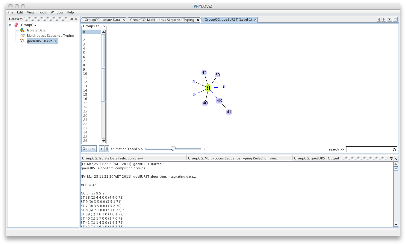
Multiple groups can be displayed simultaneously by selecting them, using the CTRL /CMD and/or SHIFT keys.

goeBURST Full MST algorithm

Using an extension of the goeBURST rules up to \(n\)LV level (where \(n\) equals to the number of loci your dataset uses), a Minimum Spanning Tree-like structure can be drawn. This is typicially used for SNP or cg/wgMLST datasets with dozens to thousand of loci.

Select goeBURST Full MST in the Compute options to draw it. Contrary to the standard goeBURST, the link statistics are not presented. After computation, double click on the goeBURST Full MST that appears under the dataset heading to visualize the result.

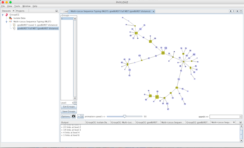
New options appear on the display: The Level selector and two new buttons Get Groups and Save Groups. The Level represents the Locus Variant level and allows the removal of all the links greater than the number represented. The user can use the up and down arrows or directly edit the number by clicking on it. The Get Groups button allows separate the display of groups that are not connected at the level chosen in order to simplify the analysis of larger datasets. This will generate a display very similar to that of goeBURST, but at a higher link level. The Save Groups creates an extra column in the isolate data with the title label goeBURST MST[\(x\)] with \(x\) being equal to the level used to create the groups.

Decreasing the Level selector, allows the user to see how clonal complexes would relate to each other at a certain level. Level 1, 2 and 3 are equivalent to calculating goeBURST at those levels (SLV,DLV and TLV respectively). The following images shows what happens to the dataset when you decrease the level. Level 4 is not displayed since no new groups are formed at that level.

At level 5 only two groups are formed in the sample dataset.

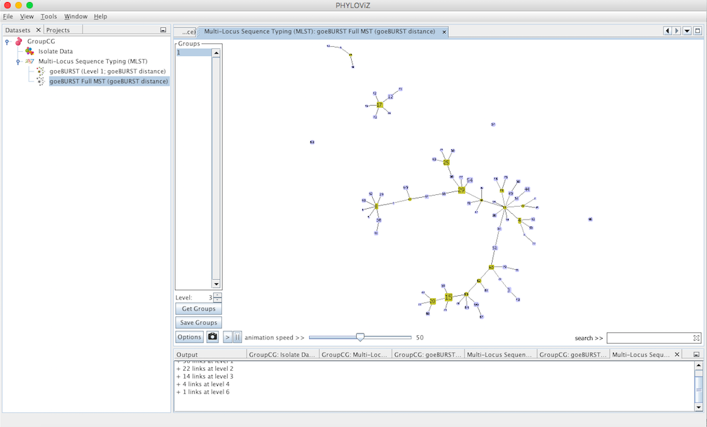
At level 3 (TLV level) some singletons appear. Level 4 is not shown since no changes were observed in the graph. This means that there are no two STs in the dataset that differ in 4 of the loci of their profiles.

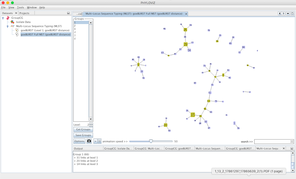
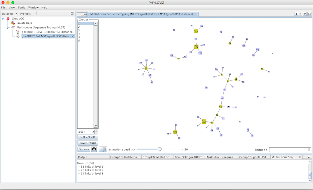
At level 2 , 6 groups appear with 4 or more STs each.

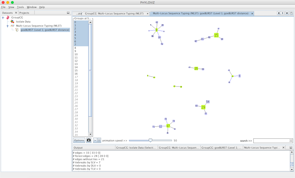
And finally at level 1, the equivalent of the most commonly used Clonal Complex definition by goeBURST, 17 groups with 2 or more STs are formed and there are 25 singletons on the dataset.

Hierarchical Clustering

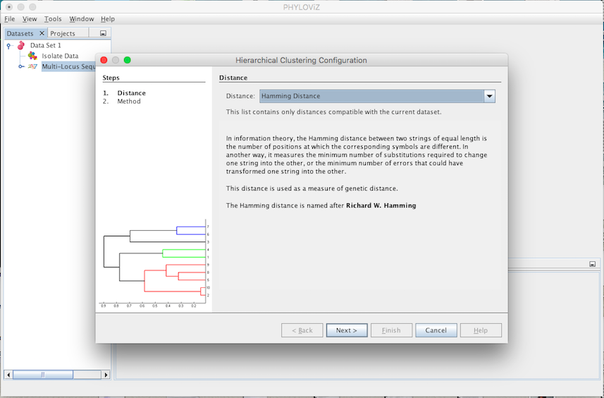
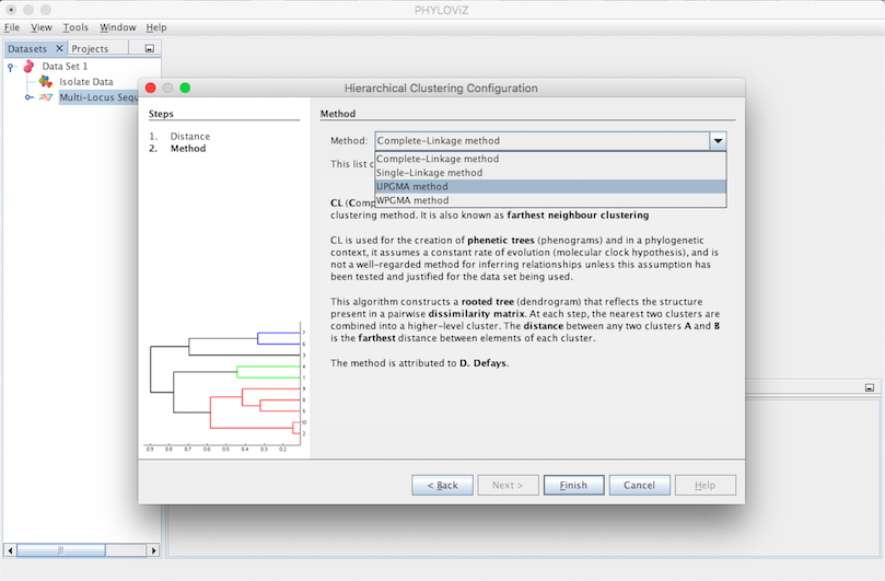
Selecting the Hierarchical Clustering opens the dialog where you can select what method you want to apply. The first step is choosing the Distance to be used. Currently the hamming distance is the only one available, but others could be implemented.

The second step is to select the Method. You can choose between complete-linkage, single-linkage, UPGMA (Unweighted Pair Group Method with Arithmetic mean) and WPGMA (Weighted Pair Group Method with Arithmetic mean). Selecting the method corresponds to selecting the criterion of minimal dissimilarity.

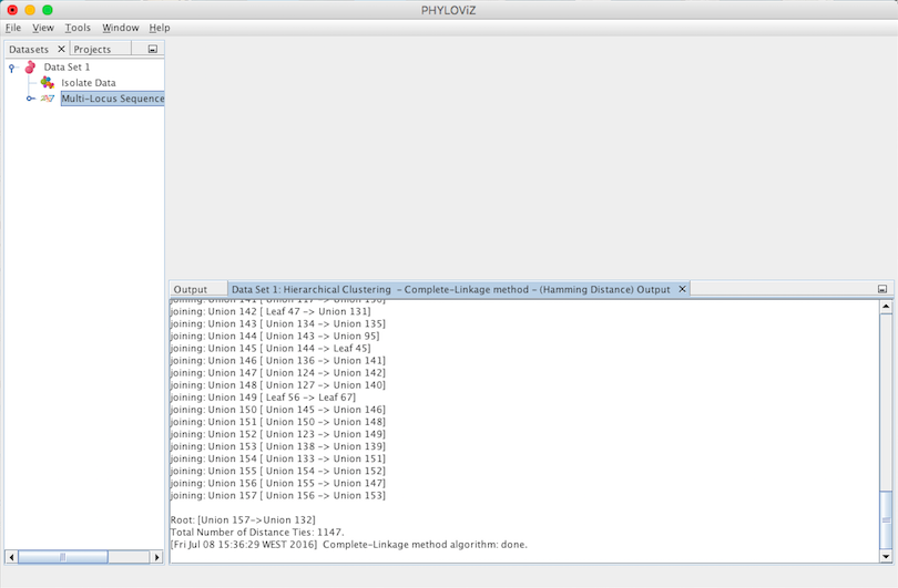
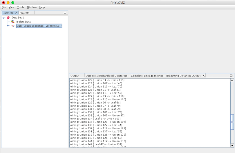
A Hierarchical Clustering Output Tab will appear and display the results of the application of the chosen method. A Leaf represents a Sequence Type and a Union represents a group that results of joining Leafs or Unions with Leafs. This process of joining is displayed step by step by the algorithm in the Output’s Tab. Finally we have the number of ties occured. The tie break applied is to always choose the first one found.

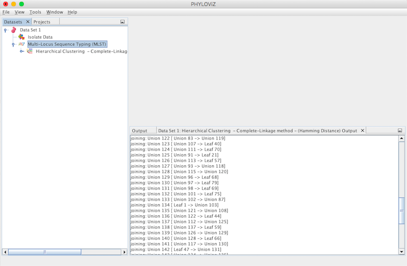
In order to display the dendogram view, it is necessary to expand the typing data on the Datasets’ tab, if it is not already expanded.

It shoud appear an icon corresponding to the hierarchical clustering computation

Double clicking on the Hierarchical Clustering item will show the display. This type of clustering is represented in the format of a dendogram. The following screenshot summarizes the output for the previous dataset. Sometimes it is necessary to fit the image to see all the display at once. To do this, please right click on the mouse over the display.

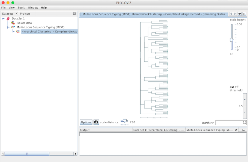
Some features were added to the visualization to improve and facilitate the analysis. These features are the following:

1. Height scale
2. Width scale
3. Options Panel
4. Search ST
5. Filter by distance (cut off threshold)
6. Export image

See section display and visualization for more information on these features.

Neighbor Joinning

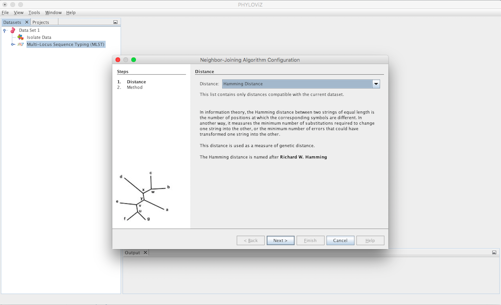
Selecting the Neighbor Joinning algorithm opens the dialog where you can select what method you want to apply. The first step is choosing the Distance to be used.

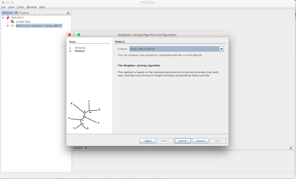
The second step is to select the Criteria of the tree branch-length minimization. You can choose between Saitou-Nei and Studier-Keppler criterion.

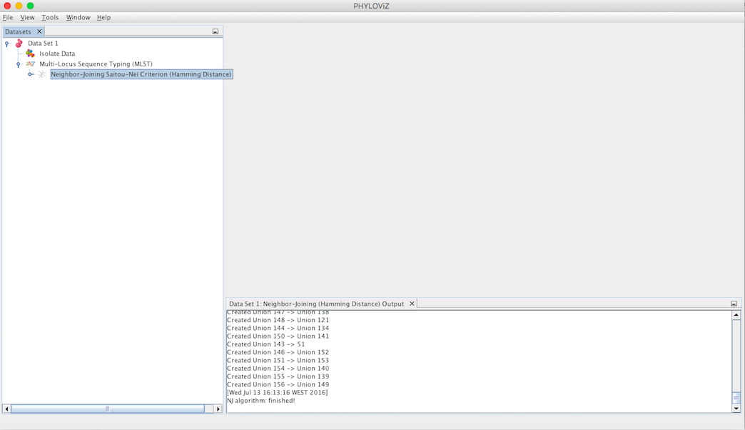
A Neighbor Joinning Output Tab will appear and display the results of the application of the chosen method. The information displayed represents the same as the Hierarchical Clustering Output Tab.

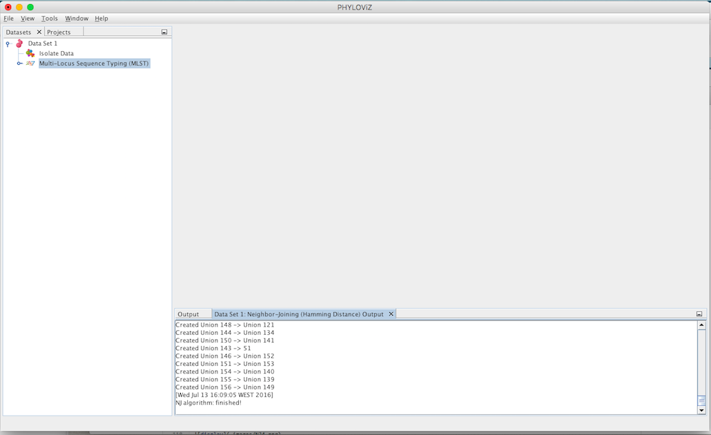
In order to display the view, it is necessary to expand the typing data on the Dataset’s tab, if it is not already expanded.

Double clicking on the Neighbor Joinning item will show the display. By default it is represented in the format of a radial tree. The following screenshot summarizes the output for the previous dataset.

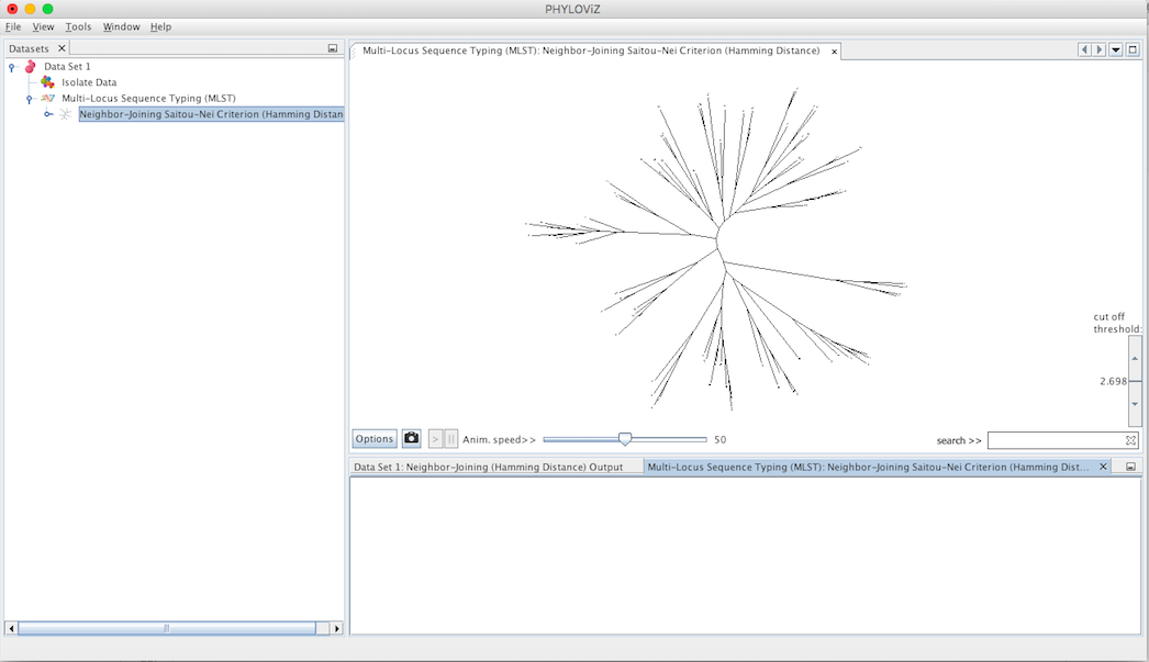
Some features were added to the visualization to improve and facilitate the analysis. These features are the following:

1. Options Panel that includes changing the tree layout
2. Search ST
3. Filter by distance
4. Export image